“How can one look [un]happy when he is thinking about the anomalous Zeeman effect?” – Wolfgang Pauli
-
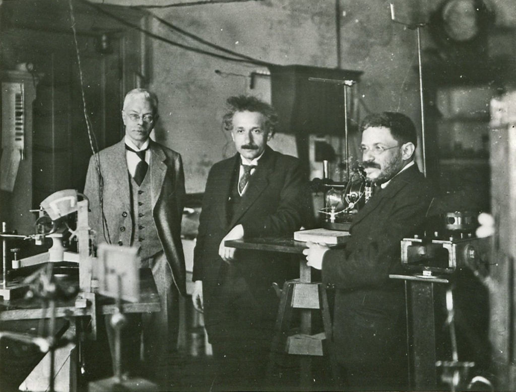
Photo: Albert Einstein (middle) and Paul Ehrenfest (right) visiting Zeeman (left) at his laboratory in Amsterdam, 1920s. This work was completed as part of the Contemporary Experimental Physics (PHYS174) course in the Pomona College Physics and Astronomy Department, by researchers Nora Anna Wu and Jacob Dong Zhang.
Abstract
In this investigation, we aimed to observe and quantify the anomalous Zeeman effect. We initially reproduced the classic laboratory setup for observing Mercury Fabry-Perot etalon fringes by camera, then attempted to extend to using 1) a more modern, advanced Fabry-Perot interferometer with a Rubidium lamp, and 2) spectrometry with Mercury.
Background theory
The Zeeman effect is a neat, observable manifestation of quantum mechanics. To understand it, it helps to first consider the hydrogen atom, for which there is only one electron. For the electron, energy levels are discretized. When an external magnetic field is applied, these levels split into multiple levels. That splitting is the Zeeman effect.
To dive deeper into the physics, the energy change between the split levels and the original ones is given by the interaction between total electron angular momentum, expressed as a magnetic dipole moment (μ) and the applied magnetic field (B).
ΔE= –μ⋅B
As a classical analog, if you hold a bar magnet near another magnet, it takes energy to anti align them, and releases energy to let them align. The energy depends on the angle between, giving rise to the dot product.
Total angular momentum may be further resolved into orbital angular momentum (L) and intrinsic “spin” angular momentum (S). Each component contributes to the magnetic moment. For orbital angular momentum, the moment is defined:
μl = -(e/2me)L = -(1/ℏ)glμbL
The first expression is simple: e is the charge of the electron, me is electron mass, and the expression is negative to indicate the negative charge of the electron. This is then defined via constants μb = eℏ/2me, the “Bohr magneton”, and gl, the “g-factor”. The g factor tells us how many μb units we have per ℏ of angular momentum.
The spin moment is defined similarly:
μs = -(1/ℏ)gsμbS
However, whereas gl = 1, gs = 2. Though spin exists to constitute necessary, “mystery” angular momenta (eg. Stern Gerlach), if we treated it as we do classic orbiting charges, we should expect a g-factor of 1. This special factor further serves to distinguish spin as something mysterious…
But no matter, we can combine these two into a single magnetic moment:
μ = -(μb/ℏ)(L + 2S)
Remembering that all these quantities are defined as vectors (how L in a classical sense is a vector), we see that μ points in a direction proportional 1L + 2S. However, in the system there is a conserved total angular momentum J = L+S. This misalignment, in the regime where the external field is not particularly strong, causes only the component of μ parallel to J to survive. Therefore, the parallel component only gives a stable, non-cancelling contribution to total energy.
If we factor all of this in, we can (after a long set of derivations) observe that there are new discretized energy levels given by
ΔE = gjμbmjB
Where mj is the quantum number specifying the projection of total angular momentum along the z axis. Now you might ask, what is gj? gj is a special g-factor known as the “Landé factor”
gj = 1+ (J(J+1) + S(S+1) – L(L+1))/2J(J+1)
The Landé factor essentially captures that information of “how much μ aligns with J“.
Returning to the energy statement, because mj takes integer steps from -J to +J, a single energy level (pre-magnetic field) therefore becomes a ladder of 2J+1 evenly spaced sub-levels, with spacing gjμbB.
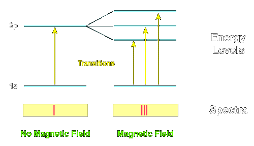
This one electron picture can be extended to a multi-electron atom, given we can find L, J, and S. These are simply the sum of the individual electron contributions. However, because completely filled electron shells have L=0 and S=0 (by symmetry), we only have to consider valence electrons.
Note that the Zeeman effect can be separated into two regimes: normal and anomalous.
For the normal Zeeman effect, S=0, indicating paired up/down spins & an effective 0 spin contribution. In this case, all of the splitting can incidentally be explained with classic electrodynamics, such that a moving charge is affected by the magnetic field in a classically consistent way. This regime correlates with a Landé factor of 1, and observed energy levels are split by increments of μbB according to mj.
On the other hand, the anomalous Zeeman effect factors in a spin contribution. This is where the name anomalous comes from! Prior to any understanding of spin, scientists exploring Zeeman splitting observed more split lines than they expected, spacings not equivalent to μbB, and different effects on different lines/atoms. As you might imagine, this was deeply confusing to scientists at the time (see Pauli quote above).
Now however, we understand that the anomalous effect is due to spin, and that what we observe through the Zeeman effect can only be explained via quantum mechanics. In this sense, the effect is a fantastic way to verify that the abstract work we do in quantum is in fact real! For this reason, in our project, we focused on observing lines that exhibit the anomalous Zeeman effect.
The easiest way to observe energy levels is by observing emission spectra. When energy in the form of photons is absorbed by an atom, energy quantization gives that both absorption and emission come in discrete energy amounts. These are manifested as the emission of photons correlating with energy level differences.
In a practical sense, we can observe these emissions via atom discharge lamps. In these lamps, gas of some atom is held in a glass tube. At each end of the tube is an electrode. When a high voltage is applied across the electrodes, free electrons accelerate toward the positive electrode. These electrons collide with atoms along the way, and if a collision transfers enough energy it will knocks an atom’s electron into a higher energy level. As it falls back to a lower energy level, the energy difference is released as a photon.
Therefore, if energy levels split per the Zeeman effect, we can observe this by observing the wavelengths of photon emissions! There are a few ways to make this observation, which is what we attempted to explore in this project.
Generating a Magnetic Field
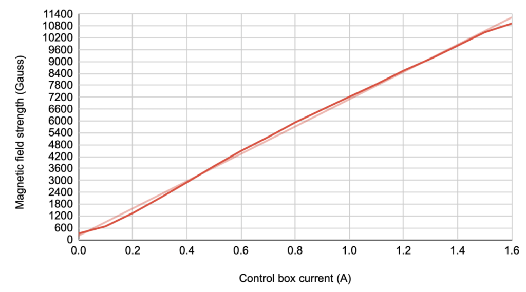
Before we were able to observe the Zeeman effect and explore different ways of doing so, we needed to ensure that we were able to generate a magnetic field. This was done via a very old electromagnet in possession by the Pomona College Physics department. The electromagnet has a control box with a current reading on it, but the accuracy of that reading was unclear. Therefore, we started by creating a calibration curve between that reading and the generated field.
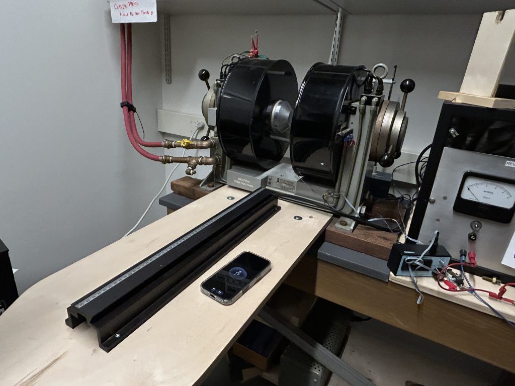
From E&M, we know that running a current through a solenoid generates a strong, uniform, axial field. To vary the strength of the field, current may be turned up or down. This creates quite a lot of Joule heating, thus the two red pipes pictured runs water through the system to carry away heat (if you hear running water in the background of our videos, that is why).
However, information about the field is not reported by the electromagnet itself. Instead, the current sent through the electromagnet is reported on the control box next to the electromagnet (pictured at right above). We used a DC magnetometer to create a calibration curve of this reported current vs. magnetic field.

This might prompt the question, why not just calculate the B field from the current reading on the electromagnet? The problem was, we were unsure that the current actually running through the coils was what was being reported by the electromagnet panel. By directly measuring the strength of the magnetic field, we could circumvent this issue. This is of aid as, when we actually took measurements of increased magnetic fields, the most straightforward measurement to note was the current reading on the box. Furthermore, we could stick the magnetometer in the specific area our discharge lamps would be located. This improved our experimental confidence in the strength of our magnetic field acting on our discharge lamp atoms.
As a final note, we confirmed our calibration curve by comparing it to a document we found sitting around in the electromagnet room created by Prof. David Tanenbaum. Our curve and his curve match up ~1 to 1, giving us greater confidence in our data.
Note: we didn’t just use his curve, as it was dated 2007. Who knows what may happen to an electromagnet in 19 years?
The curve generated by all this work is shown below:
After we had verified that our electromagnet was functioning, and that we had a way to determine magnetic field strength, we attempted to explore three methods for observing the Zeeman effect.
We started by verifying a well documented procedure for observing the Zeeman effect, imaging Mercury lines. Once that was qualitatively confirmed, we moved on to working with a Rubidium Lamp + ThorLabs scanning Fabry-Perot Interferometer, and an Oceanoptics spectrometer with the Mercury lamp. These three experiments, and their methods and results are outlined below:
Conclusion
In conclusion, we explored three ways to observe the Zeeman effect. We first confirmed the method of imaging Mercury lines. As for our second investigation using the scanning Fabry-Perot, though it was unsuccessful, we became familiar with a new optical system, and conceived theories for why it may be ineffective for this usage. Finally, our exploration of spectrometry indicated potential, but also the necessity of greater wavelength resolution.
Overall, we learned most how to choose hardware that is compatible with your physical system. We hope that this website might be helpful reference for future Zeeman-explorers, particularly for information on what not to use.